
The images, which capture tracts as small as 30 square meters, offer a surprising picture of some trends in land cover. For instance, they indicate that the rate of farm land loss has slowed, while the fastest rate of urban expansion in recent decades occurred between 1984 and 1992.
But the images also confirm the ongoing-and accelerating-loss of forest land in the watershed.
The data released by the U.S. Geological Survey in December is derived from a new set of satellite images, which offer the most complete insight on land-cover trends ever produced for the Chesapeake region, according to USGS scientists.
The USGS partnered with the National Aeronautic and Space Administration and the National Oceanic and Atmospheric Administration to collect and analyze images of the Bay watershed taken from Landsat satellites during 1984, 1992, 2001 and 2006.
Data derived from these images are providing the first holistic analysis of land-cover trends for the Bay region.
“A few other places have such data, but not very many,” said Peter Claggett, a USGS geographer and data manager with the Chesapeake Bay Program.
Understanding and predicting landscape change has been central to the Bay’s restoration since the 1980s. The amount of forest cover, farm fields, and urban and suburban areas directly affects the amount of pollution that enters local waterways and also determines how well green spaces can offset the problem.
The Bay Program is using the new data in its watershed model, a sophisticated computer model that is helping to set pollution limits, or total maximum daily loads, for the Bay and its rivers.
“If you want to get the model right, you have to get land use right,” said Lewis Linker, the Bay Program’s modeling coordinator. “Land cover is the foundation.”
The Bay Program first acknowledged the importance of land use in the 1987 Bay Agreement, which called on the states to better manage development.
Nonetheless, the region until now has never had a consistent method of tracing changes, relying instead on bits and pieces of data from different sources.
One effort, led by the University of Maryland, focused on the amount of impervious surface in the watershed. It produced a well-circulated fact that impervious cover increased by 41 percent between 1990 and 2000, while the human population of the watershed grew by just 8 percent during that same period.
Past efforts, though, failed to paint a broad regional picture. They captured limited portions of the watershed, depicted one specific point in time or used different technologies to interpret what they found.
As a result, even though the Chesapeake 2000 agreement called for reducing the rate of “harmful” sprawl, officials were never able to agree on a common set of data to measure changes.
“The methods weren’t comparable,” Claggett said. “It was very hard to identify trends.”
The new satellite data fill this gap. The project was intentionally organized to use consistent methods for recording and analyzing data. The result is a catalogue of regional land cover in 16 categories over 22 years, which can be compared over time to reveal trends.
“This is the baseline for looking at how the land changes, why it changes and the impact on water quality,” Claggett said.
While analysis continues, the data has already revealed initial regional trends for tree canopy, urban areas and farmland.
Tree canopy decreased in each year studied, for a total loss of 439,080 acres between 1984 and 2006. The highest rate of loss came between 2001 and 2006.
Urban areas grew by 355,146 acres between 1984 and 2006, and showed the fastest growth between 1984 and 1992.
Farm land disappeared most quickly between 1984 and 1992, at 8,700 acres per year. The loss slowed in 2001 and 2006, at rates of 2,110 acres and 941 acres per year respectively.
Surprisingly, the most dynamic factor in land cover between 1984 and 2006 appears to be timber harvest. Large areas of tree canopy, especially in southern Virginia, gave way to grass and shrubs, and then returned to tree canopy.
The USGS will continue to interpret the data and publish land-cover trends over the coming year.
The data currently are available on the Bay Program website in a set of downloadable maps. It will soon appear in a more detailed web-based format, including GIS maps.
The Landsat program, a partnership between the USGS and NASA, gathered the original images through two satellites that scan the entire Earth every 16 days from an altitude of approximately 438 miles. Landsat imagery is considered moderate resolution, but it is the highest resolution satellite imagery available through public agencies.
Each pixel in a Landsat image records an area of 30 square meters, and the Chesapeake project produced several billion of these pixels.
USGS geographer Fred Irani, who was part of the team that analyzed the images, said moderate detail is helpful in tracking large-scale trends. All of the minor or unusual variations that occur in a local setting-a building razed to a barren field or a large stormwater pond appearing in a field-are important for small-scale analyses, but not for reflecting regional trends.
“Higher resolution introduces too much ‘noise,'” Irani said. “Lower resolution can actually help with the big picture.”
Landsat captures an array of information about Earth’s reflected light that bay scientists can use to create refined land cover maps, as opposed to the more limited, photo-like images of Google Earth which are created with a smaller array of Landsat or Landsat-like information.
Irani and a team of contractors spent more than two years interpreting the reflectance values in the images-sorting them into 16 categories of land cover, such as tree canopy, wetlands, agriculture and urban areas-before producing the set of maps that summarize their findings.
Over time, the data may help to evaluate the effectiveness of watershed management. For example, land-cover changes could be studied in an area where water quality has also changed.
If the water has improved and the land cover was relatively stable, then management choices might have triggered the improvement. If water quality worsened in the face of conservation actions, a change in land cover might have overwhelmed the effort.
The data can also help to protect wildlife habitat. Public agencies and nonprofit organizations can analyze habitat loss in smaller areas of the watershed, such as the Monocacy or Shenandoah River basins, and predict where loss is most likely to occur.
“The art of using this information is to combine it with other things,” Claggett said.
Even this sweeping set of data has limits. Land cover, Claggett points out, is not the same as land use. The image of tree canopy, seen from above, will not by itself show whether those trees are part of a forest, a suburban backyard or even an urban park.
Neither is Landsat imagery well-suited to detecting sprawl. Urban areas reveal a clear footprint of highways and other paved surfaces, but dispersed suburban development is still well-mixed with tree canopy, grass and other open green areas.
To understand the full extent of residential sprawl, the Landsat images must be aligned with other data.
“This is one piece of the puzzle,” Irani said. “It doesn’t answer all the questions, but it clarifies the situation far better than it’s been up until now.”
Technical Note:
The 1984, 1992, 2001, and 2006 Landsat-derived data sets were created by MDA Federal under contract to USGS. The resulting land use maps classify the land cover into 16 classes based on the Anderson classification scheme. For more details, see the USGS Chesapeake Bay Watershed Land Cover Data Series (CBLCD) overview.
Contributor: Lara Lutz; Bay Journal
Large Images:
+ Land cover in the York, PA region in 1984
+ Land cover in the York, PA region in 2006
Further Reading:
+ Read original Jan. 2010 Bay Journal article [external link]
+ USGS Chesapeake Bay Watershed Land Cover Data Series (CBLCD) overview (pdf)
+ USGS Chesapeake Bay Activities Webpage
+ Chesapeake Bay Program
+ Landsat’s Role in Chesapeake Bay Management
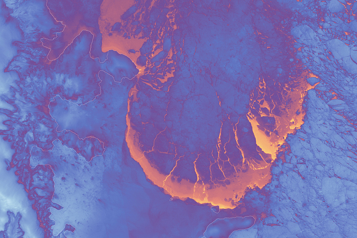
Scenes from the Polar Night
Landsat satellites have begun regularly acquiring images of ice at the poles during the winter, with enlightening results.