This afternoon Dr. James Holmquist, a Postdoctoral Research Fellow at the Smithsonian Environmental Research Center is giving a talk at #AGU17 on ways to better estimate the greenhouse gas contributions of wetlands (which can be both sinks and sources). Holmquist’s talk is taking place at 2:25 p.m. CT in Room 88-390 of the New Orleans Ernest N. Morial Convention Center.
Here is what he shared with us about his research:
Presentation Title
How much swamp are we talking here? Propagating uncertainty about the area of coastal wetlands into the U.S. greenhouse gas inventory
What are the major findings of this research?
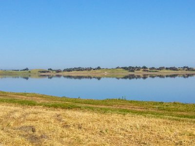
Coastal wetlands, like salt marshes, mangroves, and tidal freshwater wetlands, have the capacity to be a major sink of greenhouse gasses since they store carbon in plant biomass, and can bury it long-term in salty oxygen-poor soils. They can also emit greenhouse gasses. Because decay occurs in anoxic conditions, they can emit methane; if they erode and are lost to open water, carbon accumulated in the soil over centuries to millennia returns rapidly to the atmosphere.
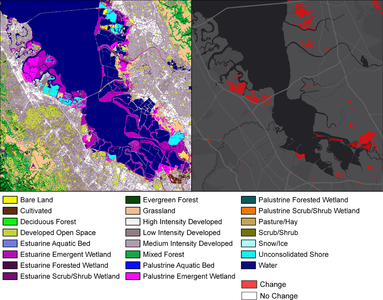
At the scale of the continental U.S., we are interested in combining maps of wetland type and wetland change with data on emission and storage associated with those types and changes. The Coastal-Change Analysis Program (C-CAP) is a Landsat-based product that allows us to do just this. However, no data set perfectly represents reality, and the C-CAP maps, the non-spatial data, and even assumptions we make, all introduce uncertainty into the inventory process.
Our research shows that the dominant contributor to uncertainty is the amount of methane emitted from the two salinity classes of wetlands currently mapped: estuarine wetlands (which includes saline and brackish wetlands) and palustrine wetlands (freshwater). We also found other factors that introduce substantial uncertainty; those were (1) the assumptions we made about the soil depth lost during erosion, (2) assumptions about the percentage of carbon lost back to the atmosphere, (3) and the rates at which stable wetlands bury carbon.
What are the implications of your findings?
Our analysis provides some context for future research targeted towards reducing uncertainty in coastal carbon monitoring, which fall into three categories: collecting more information on coastal carbon flux, developing more precise models, and improving mapping data.
For additional data collection, we have few to no measurements of the depth of soil carbon affected and the fate of carbon lost during erosion events. For model improvements, for example, uncertainty could potentially be reduced for methane fluxes by improving links between intra-wetland gradients such as plant species and biomass, tidal elevation, and salinity. For mapping data, we found that to reduce uncertainty, C-CAP’s two salinity types would need to be expanded to at least three: fresh, brackish, and saline instead of just having just two which are currently estuarine (saline and brackish) and palustrine (fresh).
This is critical because saline wetlands typically have 0 to negative emissions of methane, while brackish to fresh wetlands generally have positive emissions that are extremely variable. Better classification of these intermediate salinities would greatly reduce the uncertainty in the methane emissions.
How would you describe the importance of the Landsat-derived C-CAP product?
C-CAP is a vital program for our efforts because it is the only national-scale product that maps wetland class and change for recent decades. The C-CAP program maps two salinity classes and three vegetation types. It also registers wetland conversions to and from other land cover classes, notably registering wetland loss to open water in the Louisiana Delta following hurricanes Katrina and Rita. For our analysis, the underlying mapping data was not a dominant direct contributor to uncertainty. However, the mapping data does have limitations that could be improved with future targeted investments such as improving change detection, collecting accuracy assessment data for time steps earlier than 2006, and mapping saline, brackish, and fresh water wetlands separately.
How did you generate your unbiased wetland area estimates?
C-CAP has associated accuracy assessment data for its 2010 classifications and 2006-2010 change detection collected as part of the product’s validation (McCombs et al., 2016). This is essentially a matrix that shows counts of correct and incorrect calls for each classification. Because errors of omission and commission can be asymmetrical, and vary by land cover class, actual area can differ from mapped areas. ‘Good practices’ for estimating area from mapped area and accuracy assessment statistics are outlined by Olofsson et al., (2014) and include transforming the accuracy assessment matrix from counts to proportional areas, and summarizing the proportional areas of both agreements and omission errors for each class.
We were able to model uncertainty in land cover classes using a Monte Carlo approach. We randomly redrew all underlying data from the defined probability distributions and recalculated the inventory 1,000 times. Finally, we performed a one-at-a-time sensitivity analysis to determine the effect each estimated area, dataset, and assumption had on the overall inventory.
Why has wetland mapping traditionally been challenging?
Wetland mapping is particularly challenging because wetlands are dynamic by nature. They have standing water that shifts with seasons, tides, and weather events. Wetlands have not been highly valued from an economic standpoint historically, so much of the data we use was built for other purposes and to those purposes’ accuracy specifications. Also, collecting ground data for wetlands is expensive, labor intensive and can be invasive. In this project our goal was to determine the uncertainty inherent in using national scale data ‘as is’; it is clear from many of our group’s efforts that uncertainty can be reduced in coastal carbon monitoring, but that it will take investment in research to collect and synthesize data and generate new spatial products that accurately map gradients relevant to coastal carbon fluxes—such as salinity and inundation.
References:
McCombs, J. W., Herold, N. D., Burkhalter, S. G., & Robinson, C. J. (2016). Accuracy Assessment of NOAA Coastal Change Analysis Program 2006-2010 Land Cover and Land Cover Change Data. Photogrammetric Engineering & Remote Sensing, 82(9), 711-718.
Olofsson, P., Foody, G. M., Herold, M., Stehman, S. V., Woodcock, C. E., & Wulder, M. A. (2014). Good practices for estimating area and assessingaccuracy of land change. Remote Sensing of Environment, 148, 42-57.
Co-authors:
James Robert Holmquist
Smithsonian Environmental Research Center Edgewater
Stephen Crooks
Environmental Science Associates
Lisamarie Windham-Myers
United States Geological Survey
Patrick Megonigal
Smithsonian Env Research Ctr
Donald Weller
Smithsonian Environmental Research Center Edgewater
Meng Lu
Smithsonian Environmental Research Center
Blanca Bernal
Smithsonian Institute
Kristin B Byrd
U.S. Geological Survey
James T Morris
University of South Carolina
Tiffany Troxler
Florida International University
John McCombs
The Baldwin Group at NOAA Office for Coastal Management
Nate Herold
NOAA Charleston
Funding for this work comes from the NASA Carbon Monitoring System #NNH14AY67I
Anyone can freely download Landsat data from the USGS EarthExplorer or LandsatLook.
Further Reading:
+ Landsat at #AGU17